Outline
- Introduction
- Number Formats
- Quantization Basics
- Mixed Precision Computation
- Post Training Quantization
- Appendices
- References
Introduction
Computers approximate real numbers using finite-bit representations such as floating-point[1] which encodes numbers in a fixed-length bit sequence (e.g., FP32 uses 32 bits). Quantization for LLMs explores number formats for representing weights and activations of an LLMs, with the goal of efficiently training and deploying them. Wu et. al.[6] note three benefits of low-bit formats: (1) higher throughput of math operations, (2) reduced bandwidth requirement due to smaller word size, and (3) lower memory requirement (again, due to smaller word size) which can improve cache utilization.
Quantization involves several design choices: Which number format(s) should one choose (e.g. FP16, INT8, etc.)? Should the number format be same for weights, activations and gradients? Which quantization scheme is best (group wise, channel wise etc.)? Should the LLM be fully-trained/finetuned in low-precision or quantized post-training? In this article, I will survey quantization literature, with the aim of understanding the considerations behind each design decision.
A natural question to ask is: If quantization leads to information loss (e.g. two FP32 numbers may be represented by the same number in INT8), should we expect quantized LLMs to perform worse? Gholami et. al.[2] note that neural nets are heavily over-parametrized, and this makes their performance robust to aggressive quantization.
Number Formats
Number formats supported by hardware accelerators (such as Nvidia GPUs), are the most researched. "Support" for a number format means that Tensor Cores (processing components in a GPU which specialize in matrix-matrix multiplication) of the day allow inputs represented in that number format.
Floating Point
The "point" in floating point refers to the binary point (the dot in a binary number like 11.01 which separates its integer part from fraction). Unlike a fixed point number format which has a fixed number of bits reserved for integer and fraction (e.g. 11.01 has 2 bits each for integer and fraction, and the position of "point" is fixed), the floating point format enables the binary point to "float". This allows for a wide range of numbers that can be represented, e.g. \(1.01 \times 2^{-10}\) as well as \(1.01 \times 2^{15}\). The next few paragraphs will make this clearer.
Definition and Example
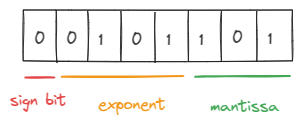
A signed \(N\) bit floating point representation has three components: \(m\) bits for the mantissa, \(e\) bits for the exponent, and 1 bit for the sign (we have \(N = 1 + e + m\)). It describes the following subset of real numbers: \[ F = \left\{(-1)^s2^{p-b}\left(1 + \frac{d_1}{2} + \frac{d_2}{2^2} + \cdots + \frac{d_m}{2^m} \right) \bigg\lvert d_i \in \{0, 1\}, s \in \{0, 1\}, p \in \{0,1,\cdots,2^e-1\}\right\} \] Here \(s\) is the sign bit, \((d_1,\cdots, d_m)\) are the \(m\) mantissa bits, and \(p\) is the integer value represented by the \(e\) exponent bits. \(b \in \mathbb{Z}\) is called the "exponent bias", typically fixed at \(2^{e-1}\). Subtracting this bias from \(p\) allows for negative exponents.
Example: Consider this number stored in an FP8 representation with a 4 bit exponent (with a bias of 7) and 3 bit mantissa (known as the FP8 E4M3 format[3]):
Floating Point Variants
There are several variants of the floating point format, depending on the total number of bits used, and how they split between the exponent and the mantissa. The IEEE 754 standard[8] describes two popular floating point formats, FP16 (known as "half precision") and FP32 ("single precision"). Read on for more details about these, and a few others:
-
16 bit: The FP16 format uses 5 exponent bits and 10 mantissa bits (going forward, I'll use the shorthand E5M10). The exponent can take any integer value in the range \([-14,15]\), which is derived by offsetting exponent bit-strings \(00001 - 11110\) (i.e., 1 to 30 in decimal), by a bias of 15. The bit-strings \(00000\) and \(11111\) have a special interpretation, which you can read more about here. The smallest representable positive number is \(2^{-24} \approx 5.96\times 10^{-8}\). The largest representable positive number (corresponding to an exponent of \(15\) and all mantissa bits 1) is \(2^{15}*\left(1+\frac{1}{2} + \cdots + \frac{1}{2^{10}}\right)\) \(= 65,504\). For contrast, the largest number that FP32 (E8M23), with just 3 extra exponent bits, can represent is \(\approx 3.4 \times 10^{38}\).
BF16 (Brain Floating Point Format) was introduced[4] by the Google Brain team. It uses E8M7 (more exponent bits and fewer mantissa bits than FP16) which allows it to represent a wider range of numbers than FP16.
- 8 bit: Nvidia's H100 GPU supports two encodings of FP8[5]: E5M2 (for quantities which require high precision such as weights and activations) and E4M3 (for gradients). Nvidia's Blackwell architecture supports a new FP8 variant called MXFP8[5] (MX stands for microscaling - read more below).
Integers
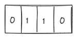
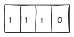
Signed integers are represented in computers using Two's Complement[7]. Say we are working in INT4 and have the following representation:
Microscaling Formats
Quantization Basics
Representable Range and Scaling
Consider conversion from FP32 (E8M23) to FP16 (E5M10). Let \(e\) denote the decimal value of exponent bits of the FP32 number less \(127\) (the FP32 bias). If \(e < -24\), the number becomes 0 in FP16 as \(2^{-24}\) is the smallest positive real number that FP16 can represent (I discuss conversion from reals to FP32, and from FP32 to lower precision formats below). Such loss of information when going to lower precision needs to be addressed. Narang et. al.[9] note that gradient values tend to be dominated by small values, and that a large number of such values may fall outside FP16's representable range of \(2^{-24}\) to \(65,504\). Figure 3. from their paper (see below), shows the distribution of gradient values for some training run. More than half the gradient values will become zero in FP16!
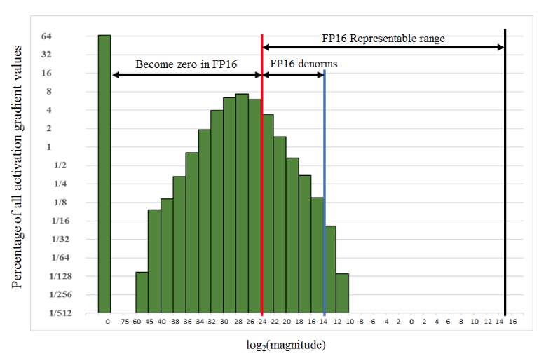
Narang et. al.[9] propose scaling up the loss by some factor, which will also scale up gradients by the same factor, and bring them into FP16's representable range. Authors recommend looking at gradient statistics, and picking a scale factor such that the maximum gradient value, when scaled, does not exceed \(65,504\) (FP16's largest representable number).
Scaling numbers in one format so that they overlap with the representable range of our destination format, will be an important consideration in all our quantization discussions (both for integers and floating point numbers). While the example above from Narang et. al.[9] used a single global scaling factor for all tensors, Peng et. al. (Appendix A2[11]) note that for larger models and formats other than FP16, we require more fine-grained scaling techniques. A simple case is where we have a different scaling factor for each tensor that is being quantized. I'll discuss this and several other variants throughout this note.
The Quantization Operation
We are interested in representing an FP32 number in a lower-precision format like FP\(x\) or INT\(x\) where \(x\) is usually one of \(\{16, 8, 6, 4\}\). The first step, common to both floats and integers, is scaling the FP32 number \(r\) by some factor \(s\) to bring it within the representable range of our destination format. Next:
-
Floating Point: See Appendix 1 for a discussion around the precision loss that may occur when we convert real numbers (infinite precision) to limited precision FP32. Such loss may also occur when we convert from FP32 to ExMy where \(x+y < 31\). Converting FP32 to ExMy involves[10]:
- Clipping the original exponent \(e\) to the range \(e_{min}, e_{max}\) representable by \(x\) bits of ExMy.
- If \(e_{min} ≤ e ≤ e_{max}\), keep the bits \(m_1m_2\cdots m_y\) (subject to some rounding; see this[10]) and discard \(m_{y+1}m_{y+2}\cdots m_{23}\). Consider the case when \(e < e_{min}\) (such numbers are called "denormal"), e.g. in FP16, \(e_{min} = -14\). Say the number is \(1.m_1m_2\cdots m_{23} * 2^{-16}\). Rewrite it to match exponent: \(0.01m_1m_2\cdots m_{23} * 2^{-14}\). For FP16, the \(10\) mantissa bits we'll use are \(01m_1m_2\cdots m_8\). In both cases, we lose precision due to lost mantissa bits.
-
Integer: When quantizing to a \(b\) bit integer format INT\(b\), our objective is to map the FP32 \(r\) to an integer in the range \(\left[-2^{b-1}, 2^{b-1} - 1 \right]\), e.g. \([-128, 127]\) for INT8. We first apply an affine transformation on \(r\) (see Section 3.1.1[6]) to get \(s\cdot r + z\), where \(s\) is the scale factor, and \(z\) is called the zero point. Next, we round the scaled and shifted \(r\) to the nearest integer, and then clip the resulting value to within the range of INT\(b\). The quantized number is: \[ \text{clip}\left(\text{round}(s\cdot r + z), -2^{b-1}, 2^{b-1} - 1 \right) \]
Mixed Precision Computation
Our baseline number format for all neural net computations is FP32. However, as we move to lower precision formats (FP16/8/4, INT8/4), using higher precision for some computations and data, may help us preserve accuracy. Narang et. al.'s paper Mixed Precision Training[9] showed the efficacy of this idea for training neural nets in mixed FP16/FP32 formats. I'll discuss the key techniques proposed by the authors, and follow it up with a discussion on hardware support for mixed precision computation.Key Ideas
-
FP32 Master Copy of Weights: We start with the original weights in FP32 (the "master" copy), and clone into an FP16 version. During forward and backward pass, we use FP16 weights and maintain gradients and activations in FP16. However, at the end of the backward pass, we update the FP32 master weights, and use them to initialize FP16 weights for the next training step. Authors note two reasons for doing so: (1) gradient updates (learning rate times gradients) may become 0 in FP16 (i.e. they are smaller than \(2^{-24}\)), and so by updating the FP32 weights, we may preserve very small updates; (2) if weights are large relative to updates, the updates might be right shifted to 0 if we were to add them to FP16 weights (e.g. in FP16, \(90.0 + 0.03\) will just be \(90.0\)).
-
Loss Scaling: We scale the loss to ensure gradients are in FP16's representable range. See above for more on this.
- Accumulator Precision: When computing a vector dot product, the individual products may be so small that they underflow in FP16 (i.e. map to 0). To fix this, the authors propose accumulating intermediate vector product sums in FP32 (i.e. an FP16-FP16 product is cast to FP32 and added to the intermediate FP32 sum using FP32 addition). We can later convert the sum back to FP16 for other computations. We can also have cases where intermediate calculations are too large for FP16 (e.g. in case of reductions such as a vector sum), and in such cases as well the authors propose using FP32 accumulators.
Tensor Cores
TODO: Tensor cores
As noted in the Introduction, quantization involves several design decisions that are largely orthogonal. In this article, I’ll organize quantization methods based on when they are applied during a model’s development lifecycle. This leads to three broad categories: Post-Training Quantization (PTQ), Quantization-Aware Training (QAT), and Fully Quantized Training (FQT). For each category, I’ll highlight commonly used techniques and the specific design choices they entail.
Post Training Quantization
LLM.int8()
Dettmers et. al.[13] propose a method to use mixed INT8 and FP16/32 to perform the matrix multiplication component (the \(XW\) in \(Y = XW + b\)) of select affine layers in LLMs. The affine layers they pick are those in the MLP block, and the QKV projection layers in the attention block. In their own words:
The LLM.int8() method is the combination of absmax vector-wise quantization and mixed precision decomposition.
Let us parse the technical terms used in this quote, and see how they are used to implement mixed INT8/FP16 matrix multiplication in LLM.int8().
-
Absmax Quantization: To quantize an FP16 tensor (of any dimension) \(X_{f16}\) to INT8, we first scale it to bring it within the INT8 range \([-128,127]\), and then round it to the nearest integer. In the Absmax method, the scale factor is \(127\) divided by the absolute maximum element of the tensor \(X_{f16}\). \[ X_{i8} = \left\lfloor \frac{127\cdot X_{f16}}{\max_j\left(\lvert X_{f16}^{(j)}\rvert\right)} \right\rceil \]
-
Vector-wise Quantization: Let \(X_{f16} \in \mathbb{R}^{t \times h}\) and \(W_{f16} \in \mathbb{R}^{h \times o}\) represent the inputs to an affine layer, and its weight matrix respectively, in FP16. To perform matrix multiplication in INT8, we first need to quantize \(X_{f16} \to X_{i8}\) and \(W_{f16} \to W_{i8}\). We can use two Absmax style scaling factors, \(\max_j\lvert X_{f16}^{(j)}\rvert\) and \(\max_j\lvert W_{f16}^{(j)}\rvert\). Vector-wise Quantization increases scaling granularity by using an independent Absmax scaling factor for each row of \(X_{f16}\) and for each column of \(W_{f16}\). Let \(c_{x_{f16}} \in \mathbb{R}^{t \times 1}\) and \(c_{w_{f16}} \in \mathbb{R}^{1 \times o}\) be those scaling factors. To perform \(X_{f16}W_{f16}\) in INT8:
- We mutiply scale factors to rows of \(X_{f16}\) and columns of \(W_{f16}\), and round elements to nearest integer, to get \(X_{i8}\) and \(W_{i8}\).
- Compute INT8 matrix multiplication, while accumulating in INT32 to get \(C_{i32} = X_{i8}W_{i8}\).
- Dequantize back to FP16 by scaling down \(C_{i32}\) by the cross product \(c_{x_{f16}} \otimes c_{w_{f16}}\), to get the final result: \[ X_{f16}W_{f16} \approx \underbrace{\frac{1}{c_{x_{f16}} \otimes c_{w_{f16}}}}_{S_{f16}} C_{i32} \] We need to dequantize the output as all computations other than matrix multiplications inside select affine layers, will be performed in FP16 and will require FP16 activations.
-
Mixed Precision Decomposition: Authors observe that a small percent of input feature dimensions (specifically, 0.1% of columns of \(X\)) tend to have large magnitude features (authors define large as \(≤ 6.0\)). Since Vector Quantization computes row-wise scaling factors, a large value in a row will determine its scaling factor, and can cause other smaller values in the row to underflow in INT8. To avoid this, the authors propose decomposing \(XW\) into two matrix multiplications: (1) one with just the outlier \(X\) columns, performed in FP16, and (2) another with non-outlier \(X\) columns, performed in INT8 usign Vector Quantization as described above. Let \(O\) be the set of such outlier input column indices. Then authors propose the following decomposition of \(XW\): \[ X_{f16}W_{f16} \approx \sum_{h \in O}X_{f16}^hW_{f16}^h + S_{f16}\sum_{h \notin O}X_{i8}^hW_{i8}^h \] This decomposition is made clearer in the example in Figure 2. from the paper below:
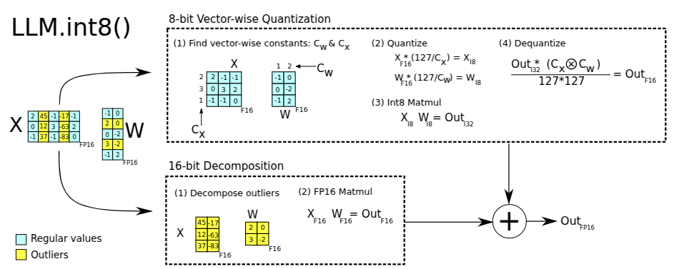
Dettmers et. al.[13] (Figure 2): Decomposition of \(X\) into two sub-matrices (based on its outlier columns). Corresponding rows of \(W\) also decouple from the rest.
Overheads and Inference Speed: Quantizing inputs and dequantizing outputs incurs computation overheads which impact speedups relative to FP16. Authors note (see Appendix D.1 of paper) that raw INT8 matrix multiplication in the first LLM hidden layer, with model dimension of \(5,140\) is 2x faster than in FP16, but only 1.6x faster when we include quantization and dequantization.
SmoothQuant
Xiao et. al.[14] note that LLM.int8()'s Mixed Precision Decomposition approach is hard to implement efficiently on GPUs. In LLM.int8(), Dettmers et. al. observed that 0.1% of input dimensions (also called channels) of \(X_{f16} \in \mathbb{R}^{t \times h}\) had outliers (here \(t\) is known as the sequence or token dimension). Their solution decoupled \(X_{f16}\) into two sub-matrices with outlier channels and non-outlier channels (with only the latter using INT8 matrix multiplication with weights). They used Vector-wise Quantization on the non-outlier sub-matrix of \(X_{f16}\), with scale factors computed along the token dimension (i.e. one factor per row).
Can we use channels as the scaling dimension instead of tokens? Instead of decomposing \(X_{f16}\) into outliers vs. non-outliers, and then scaling the non-outlier sub-matrix along the token-dimension, can we avoid decomposing \(X_{f16}\), and just scale entire \(X_{f16}\) along the channel dimension? This is theoretically possible as Xiao et. al. observed that if a channel has an outlier, it consistently has large values across all tokens, and so if we were to have one scale factor for that channel, it would not push any values to underflow. However, they note that the reason this isn't done is because hardware considerations do not permit an efficient implement of channel-wise scaling. Specifically, they note that INT8 GEMM kernels which execute on Tensor Cores only allow scaling along outer dimensions (the token dimension \(t\) for \(X\), and the channel dimension \(o\) for \(W\)), after the matrix product \(X_{i8}W_{i8}\) has been computed. Authors conclude that per-channel activation quantization is infeasible and propose an alternative method:
... SmoothQuant smooths the activation outliers by offline migrating the quantization difficulty from activations to weights ...
Activations are harder to quantize than weights due to the presence of outlier values (weight values are usually uniform). The basic idea behind SmoothQuant is to scale down activations \(X\) by dividing by a per-channel "smoothing factor" \(s \in \mathbb{R}^h\) and scale up corresponding weights \(W\) by an equivalent amount such that the product \(XW\) remains unchanged. \[ Y = XW = \left(X \text{diag}(s)^{-1}\right)\left(\text{diag}(s)W\right) \] The effect of this scaling is that the magnitudes of outliers in \(X\) are reduced, making quantization easier than before. This comes at the cost of introducing outliers in \(W\) though, and we need to somehow strike a balance.
Choice of Smoothing Factor
-
A simple choice for \(s\) is Absmax style channel-wise factors, i.e. \(s_j = \max \left(\lvert X[:,j]\rvert\right)\) for \(j = 1,2,\cdots h\). Authors note that this choice "pushes all difficulty to the weights" making quantization of \(W\) harder.
-
To strike a balance, authors propose a hyperparameter migration strength \(\alpha\), and propose the following formula for smoothing factor (with \(\alpha = 0.5\) proving optima for most models): \[ s_j = \frac{\max \left(\lvert X[:,j]\rvert\right)^\alpha}{\max \left(\lvert W[j,:]\rvert\right)^{1-\alpha}} \]
-
Authors note that since activations \(X\) are produced from some previous layer, this scaled smoothing operation can be fused into parameters of that layer prior to using the model for inference. We can estimate these scales using calibration datapoints from the pre-training dataset. To quantize weights in the smooth scaled LLM, authors use per-tensor scaling factors. For quantizing activations, authors use three variants in their experiments (all of which scale along the outer token-dimension of \(X\)): (1) per-token dynamic ("dynamic" means the scaling factor is not pre-computed - it is computed using inference time activation statistics), (2) per-tensir dynamic, and (3) per-tensor static (scaling factors are computed from some calibration dataset).
GPTQ
Frantar et. al.'s[15] GPTQ is a weight-only quantization method. During inference, activations are not quantized, and instead weights are dequantized back to FP16 for computation. Despite dequantization related overheads, GPTQ achieves speedups relative to FP16. This is because inference involves matrix-vector products (between weight matrices and query vectors) - a memory bound operation - and GPTQ kernels have to make fewer memory accesses (due to weights being stored in lower precision than FP16).
Layer-wise Quantization: For each linear layer with weights \(W\), GPTQ assumes some fixed quantization grid, and estimates quantized weights \(\hat{W}\) by minimizing the following reconstruction error (with \(X\) drawn from a calibration dataset): \[ \text{argmin}_{\hat{W}} \left\lvert \left\lvert WX - \hat{W}X \right\rvert \right\rvert_2^2 \] The authors note that the calibration dataset need not be task-specific. In their experiments, the calibration dataset consisted of just 128 random 2,048 token sequences from the C4 dataset (which itself was created from randomly crawled websites). The reconstruction error optimization was performed using authors' technique Optimal Brain Quantization, which I will not discuss in this article.
FP8 PTQ
Shen et. al.[16] recommend a PTQ scheme in which they use E4M3 as the only format. They perform per-channel scaling for quantizing weights, and per-tensor scaling for activations. They apply SmoothQuant with \(\alpha = 0.5\) to make activation quantization easier. With this setup, they achieved accuracies on par with their FP32 baseline, on at least 96% of test datapoints (see Table 2 from paper), across a variety of NLP tasks.
PTQ in Practice
In practice, we use a combination of some of the approaches discussed above. For example, in vLLM's recipe for INT W8A8:
- We use SmoothQuant to make activations easier to quantize to INT8. We need a calibration dataset to estimate smoothing factors, and vLLM recommends 512 sequences of 2,048 tokens each, drawn from a dataset that matches inference data distribution.
- We quantize the weights to INT8 using GPTQ (with the same calibration dataset that we used for smoothing).
- To quantize activations to INT8 during inference, we use dynamic per-token scale factors.
In vLLM's example FP8 W8A8 recipe, we perform per-channel static quantization for weights of all Linear layers, and per-token dynamic quantization for activations. Thus, we do not require any calibration dataset (note: we would require a dataset if we were to use SmoothQuant as well).
Appendices
Appendix 1: Infinite to Limited Precision Conversion
For simplicity, I'll just discuss positive numbers in this section. Consider a real number \(n = 0.1729\). First, we want to write it in the form \(n = m * 2^e\). Without constraints on \(m\) and \(e\), there are many ways to write a number in this form, e.g. \(3.5 = 7 * 2^{-1} = 1.75 * 2^1\). We settle on the form where \(2^{-1} ≤ m < 0\). \[ n = m * 2^e \\ \implies \log_2n = \log_2m + e \\ \implies e = \log_2n - \log_2m \] Because of the constraints imposed on \(m\), we have \(-1 ≤ \log_2m < 0\). This gives us: \[ \log_2n ≤ e < \log_2n + 1 \\ \implies e = \lfloor \log_2n \rfloor + 1 \] For our example, \(e = -2\) and \(m = n / 2^e = 0.6916\). Next we'll translate this form \(m * 2^e\) into its binary representation. We start with FP32 (E8M23 with a bias of 127), where a 32-bit binary representation looks like: \[ \underbrace{s}_{\text{sign} \\ \text{bit}} \big \lvert \underbrace{e_1e_2\cdots e_8}_{\text{exponent bits}} \big \rvert \underbrace{m_1m_2\cdots m_{23}}_{\text{mantissa bits}} \]
Mantissa Bits: The mantissa \(m\) equals the value represented by the binary string \(1.m_1m_2\cdots m_{23}\) (the leading 1 is thus implicit and not stored in the floating point representation). However, the value of this binary string lies within \([1, 2)\) while \(0.5 ≤ m < 1\). Therefore, to map \(m\) to this string, we make these adjustments: \(m = m*2 = 1.3832\) and \(e = e-1 = -3\). The number we want to represent using bits \(m_1m_2\cdots m_{23}\) then is \(m-1 = 0.3832\) (taking away the implicit leading 1). We can do that by shifting the number \(0.3832\) left by 1 bit at a time (repeating this 23 times), and recording the post-shift leading bit. Here is a code snippet to do this:
mantissa_fraction = 0.3832
m_scaled = mantissa_fraction
mantissa_bits = 0

for _ in range(24):
    # left shift by 1 bit
    m_scaled *= 2

    # extract leading bit
    bit = int(m_scaled)

    """
    extend the bit string (left shift makes least
    significant bit 0 and then we OR with the
    extracted bit)
    """
    mantissa_bits = (mantissa_bits << 1) | bit

    # remove leading bit
    m_scaled -= bit

print(f"{mantissa_bits:023b}")
Precision Loss: In the example above, if we did not stop after 23 iterations, we could've extracted more non-zero bits, and our resulting value would've been closer to the real \(0.1729\). Restricting mantissa to 23 bits results in loss of this information (also called "precision loss").
Exponent Bits: Let \(p\) denote the decimal value represented by the exponent bits. Then we have \(p = 127 + e = 124\).
References
- What Every Computer Scientist Should Know About Floating-Point Arithmetic
- Gholami et. al. (2021), A Survey of Quantization Methods for Efficient Neural Network Inference
- Micikevicius et. al. (2022), FP8 Formats for Deep Learning
- Wang and Kanwar (2019), BFloat16: The secret to high performance on Cloud TPUs
- Nvidia, Using FP8 with Transformer Engine
- Wu et. al. (2020), Integer Quantization for Deep Learning Inference: Principles and Empirical Evaluation
- Wikipedia, Signed Number Representations
- Wikipedia, The IEEE Standard for Floating-Point Arithmetic (IEEE 754)
- Narang et. al. (2018), Mixed Precision Training
- Corsix, The many ways of converting FP32 to FP16
- Peng et. al. (2023), FP8-LM: Training FP8 Large Language Models
- Gong et. al. (2024), A Survey of Low-bit Large Language Models: Basics, Systems, and Algorithms
- Dettmers et. al. (2022), LLM.int8(): 8-bit Matrix Multiplication for Transformers at Scale
- Xiao et. al. (2022), SmoothQuant: Accurate and Efficient Post-Training Quantization for Large Language Models
- Frantar et. al. (2022), GPTQ: Accurate Post-Training Quantization for Generative Pre-trained Transformers
- Shen et. al. (2023), Efficient Post-training Quantization with FP8 Formats